
Basics
我们首先来看一下Shannon是如何定义加密的:
Schannon cipher 是一个加密方案(encryption scheme)$\Pi := (E,D)$ ,作用于$(\mathcal{K},\mathcal{M},\mathcal{C})$上,其中:
- $\mathcal{K}$ 是一个有限的加密密钥集合。
- $\mathcal{M}$ 是一个有限的消息集合。
- $\mathcal{C}$ 是一个有限的密文集合。
- $E: \mathcal{K} \times \mathcal{M} \to \mathcal{C}$ 是加密函数。
- $D: \mathcal{K} \times \mathcal{C} \to \mathcal{M}$ 是解密函数。
- 并且满足Correctness property:$\forall k \in \mathcal{K},\ m \in \mathcal{M} :\ D(k, E(k, m)) = m$。
我们来看一个很简单的例子:One-time-pad (OTP)。
- $\mathcal{K} = \mathcal{M} = \mathcal{C} := \{0,1\}^L$ with $L$ as a fixed length $\geq 1$.
- $E(k, m) := k \oplus m$
- $D(k, c) := k \oplus c$
(这里的$\oplus$表示的是xor运算。)
注意到:
所以OPT是一个Schannon cipher。
Definition 1: (Perfect Ciphertext Indistinguishability / perfect secrecy / perfect security)
一个定义在 $(\mathcal{K}, \mathcal{M}, \mathcal{C})$ 上的 Shannon cipher $\Pi = (E, D)$,满足密文完全不可区分(has perfectly indistinguishable ciphertexts)(或者说是绝对安全 perfectly secure的),当
其中概率是针对密钥的分布而言,$k$ 是一个随机变量。
我们会假设每个密钥 $k$ 都是从 $\mathcal{K}$ 里uniformly挑选的,即每个密钥被挑选的概率都等于 $\frac{1}{\mathcal{K}}$。
设
为可以将m加密成c的密钥数量,那么我们可以将定义里的等式重新重新表述为:
也就是说对于任意2个明文和1个密文,都存在同样多的密钥可以将这两段密文都加密成这段密文。
Theorem 1:
The one-time pad (OTP) is perfectly secure.
证明:
Given an OTP, for all $m \in \mathcal{M}$ there is exactly one unique $k \in \mathcal{K}$ such that $E(k, m) = c$. It follows that $N_{m,c} = 1$,因为
- 存在:There is at least one key $k := c \oplus m$ with $E(c \oplus m, m) = c \oplus m \oplus m = c$.
- 唯一:Assuming two keys $k_0, k_1 \in \mathcal{K}$ exist where $E(k_0, m) = E(k_1, m) = c$:
所以有:
. $\square$
Theorem 2:
如果$\Pi = (E, D)$是绝对安全的(perfectly secure),那么有 $|\mathcal{K}| \geq |\mathcal{M}|$。
证明:
我们假设 $|\mathcal{K}| < |\mathcal{M}|$,并任意选择一段明文$m_0$和一个密钥$k’$。设$c := E(k’,m_0)$,那么有
设
为c所有可能的解密结果。选择$m_1\in \mathcal{M}\backslash S$ (这个集合非空是因为 $|S| \leq |\mathcal{K}| < |\mathcal{M}|$),那么就有
a contradiction. $\square$
该如何理解这个定理呢?
其主要说明的就是当密钥空间小于信息空间时,可能会对于有些密文只存在一个(可能的)对应的明文。
然而在实际情况里,一直要求密钥空间大于信息空间其实不太现实,因为我们需要各方各面都传输大量的信息。这就导致Shannon提出来的这个perfect secrecy概念不够实用(practical)。
其根本的原因是,shannon提出来的概念着重于杜绝所有潜在的威胁。但实际上对我们来说,有些威胁是可以接受的:比如说质因数分解很大的数需要大量的计算资源与时间,对我们很难造成什么实质性的威胁。又或者是我运气够好,可以一下子猜到密码。
所以说我们实际追求的是无法以不可忽略的(non-negligible)概率被高效(efficiently)破解的高效加密算法,。
What we would like to have are efficient encryption schemes that cannot be broken “efficiently” with a “non-negligible” probability.
比如说质因数分解,它的理论成功概率很高,但是效率非常低,所以可以被忽视。而猜密码这种方法的成功概率太低了,所以也不需要理会。
重新表述一下就是:“不存在一个算法可以在时间T内以p的概率成功破解我们的加密算法”。
Definition 2 (Polynomially-bounded):
A function $f : \mathbb{Z}_+ \to \mathbb{R}$ is called polynomially-bounded if there exist $c, n_0 \in \mathbb{N}$ such that for all integers $n \geq n_0$, we have
Definition 3 (PPT algorithm):
An algorithm is called efficient, if its runtime as a function of its input length is polynomially-bounded.
We call this algorithm a probabilistic polynomial time (PPT) algorithm.
就其实efficient和PPT是一个意思。
Definition 4 (Efficiently sampleable):
A set $S$ is efficiently sampleable if there is a PPT-algorithm that is able to sample an element from it uniformly and randomly.
For such a sampling, we use the notation $s \xleftarrow{R} S$.
Definition 5 (Negligible):
A function
is called negligible if
$f$的值会无限小。
例子:$\frac{1}{2^n},\quad \frac{1}{n^{\log n}}$,the probability of randomly choosing a specific key from a set of $2^n$ $n$-bit keys
Definition 6 (Super-poly):
A function $f : \mathbb{Z}_+ \to \mathbb{R}$ is called super-poly if $\frac{1}{f}$ is negligible.
翻译一下:
对于所有的 $c \in \mathbb{N}$ 都存在一个 $n_0 \in \mathbb{Z}_+$使得 for all integers $n \geq n_0$, we have :
例子:The runtime of an algorithm enumerating all $n$-bit keys to possible ciphertexts for a message $m$ by calculating $E(k, m)$ for all $2^n$ keys is super-poly.
Let $c \in \mathbb{R}_+$ be a constant,
be negligible functions,
be polynomially-bounded functions, and
be super-polynomial functions.
Then:
通常我们会定义2个参数:
Security parameter$\lambda$: A positive integer.System parameter$\Lambda$: A bit string.
$\lambda$ is chosen when a cipher is deployed. 一般来说,$\lambda$ 的值越大,密码系统的安全等级越高。较高的值通常与较长的密钥相关联,同时对加解密操作 $D$ 和 $E$ 的性能带来负面影响。
而$\Lambda$ is not chosen but determined by $\lambda$ for a specific cipher. 比如说,$\lambda$可能表示模数 $n$ 的位长度(length in bits),$n$本身则为成为System parameter$\Lambda$。
这两个参数都是公开的。
The parameterization applies the key, message and ciphertext spaces
Definition 7 (efficient algorithm):
Let $A$ be an algorithm that takes as input a security parameter $\lambda \in \mathbb{Z}_{\geq 1}$, as well as other parameters encoded as a bit string $x \in \{0,1\}^{\leq p(\lambda)}$ for some fixed polynomial $p$.
We call $A$ an efficient algorithm if there exist a poly-bounded function $t$ and a negligible function $\epsilon$
such that for all $\lambda$ and $x$, the probability that the running time of $A$ on input $(\lambda, x)$ exceeds $t(\lambda)$ is at most $\epsilon(\lambda)$.
翻译一下:A的输入为一个 security parameter $\lambda \in \mathbb{Z}_{\geq 1}$, 以及被 encoded as a bit string $x \in \{0,1\}^{\leq p(\lambda)}$ (for some fixed polynomial $p$)的其他的parameters。
Definition 8 (computational cipher):
A computational cipher is a pair of efficient algorithms $\Pi := (E,D)$ such that:
- $k \in \mathcal{K}$ is an encryption key.
- $m \in \mathcal{M}$ is a message.
- $c \in \mathcal{C}$ is a ciphertext.
- $E : \mathcal{K} \times \mathcal{M} \rightarrow \mathcal{C}$ is the encryption algorithm.
- $D : \mathcal{K} \times \mathcal{C} \rightarrow \mathcal{M}$ is the decryption algorithm.
- $\mathcal{K}, \mathcal{M}$ and $\mathcal{C}$ are finite spaces.
computational cipher的定义其实和Shannon cipher就只差了一个 efficient algorithms 的条件。
当然在现实生活中,传输数据时会产生各种随机的噪音,所以$E$ 可以是 non-deterministic。在这种情况下我们会引入一个新的参数randomness:$r \in \mathcal{R}$ ,并且用
表示(受随机数的影响的)加密后的结果。
(这里箭头上的$R$就只是表面当前考虑的是受随机数的影响的加密)
而correctness requirement也需要随之改写成:
(即就算受随机数的影响,也需要可以成功解密出来。感觉跟coding theory很像。)
当$E$ 是 deterministic 的时候,我们会把$\Pi = (E,D)$ 叫作 deterministic cipher。(比如说OTP)
一个deterministic cipher显然是Shannon cipher。
之前我们定义的 Perfect Ciphertext Indistinguishability 是这样的:
而我们希望将这个定义推广到可以适应所有的 predicate $\phi$(一个判断函数,输出结果只为true或者false。也就是一个从$\mathcal{C}$ 映射到$\{0,1\}$的函数。比如说判断“密文的前4位是否全为0”。):
给这个式子引入一个误差(a negligible chance for an adversary to break our scheme by demanding)就会变成:
这个便是Statistical Ciphertext Indistinguishability的定义。
而所谓的Computational Ciphertext Indistinguishability便是在此基础上继续要求 predicate $\phi$ 是efficient。
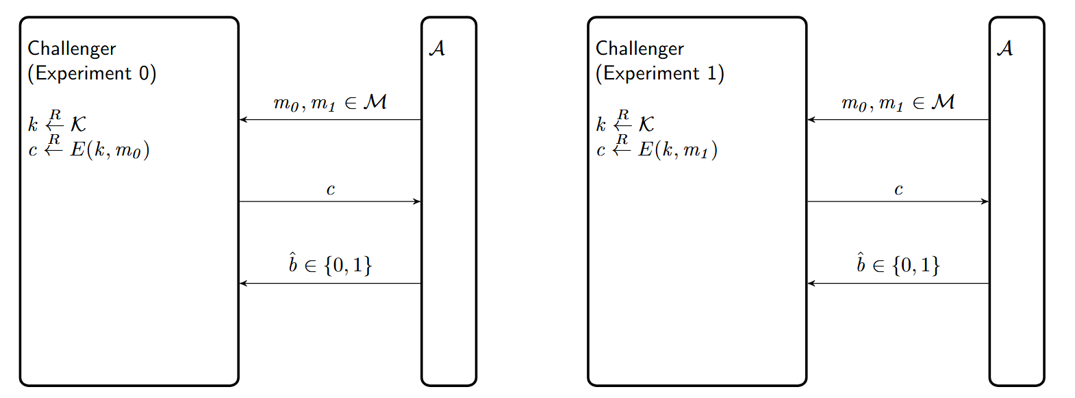
Attack Game
我们通常会用一个Attack Game来形式化定义安全性。会有一个Adversary $\mathcal{A}$,如果他的输出不同于任何”trivial attack”(比如说随机猜测),那么我们就说他破解(break)了我们的加密。我们会用$\mathcal{A}$’s advantage 来衡量他对我们的加密有多大的影响。
Attack Game 1 (Ciphertext Indistinguishability):
For a given cipher $\Pi = (E, D)$ defined over $(\mathcal{K}, \mathcal{M}, \mathcal{C})$ and for a given adversary $\mathcal{A}$, we define two experiments.
For $b \in \{0,1\}$, Experiment $b$ proceeds as follows:
The adversary computes $m_0, m_1 \in \mathcal{M}$ of the same length and sends them to a challenger.
The challenger computes
and sends $c$ to the adversary.
The adversary outputs a bit $\hat{b} \in \{0,1\}$.
Let $W_b$ be the event that $\mathcal{A}$ outputs 1.($\mathcal{A}$在实验b的时候输出1)
图示:
Definition:
We define $\mathcal{A}$’s ciphertext distinguishing advantage or semantic security advantage as
Definition 9 (Ciphertext Indistinguishability):
A cipher $\Pi := (E, D)$ has (computationally) indistinguishable ciphertexts,
if $SC_{adv}[\mathcal{A}, \Pi]$ is negligible for all PPT adversaries $\mathcal{A}$.
如果对于所有adversaries $\mathcal{A}$都有:
那么它一定是(computationally) indistinguishable ciphertexts。
例子:
Trivial attacks
如果$\mathcal{A}$永远输出1,那么
如果$\mathcal{A}$通过扔硬币选择输出,那么
如果挑选2条一样的明文,那么advantage也等于0,因为不可能通过任何手段可以判断出来到底加密的是哪条信息,所以只能猜,也就是$|\frac{1}{2} - \frac{1}{2}| = 0$。
假如这样设计一个加密:$E(k, m) := (\text{parity}(m), E’(k, m))$,即加密结果包含2个信息,第一个是明文$m$的奇偶性,第二个是真正的加密内容,那么就会存在一个 adversary with advantage 1:
- $\mathcal{A}$挑选2个明文,一个的parity等于1,一个的等于0.那么他就可以通过$E(k, m)$的第一个component的值(parity)来判断明文到底是那条。
对于perfectly secure ciphers,所有的adversary has advantage 0 。
如果我们让challenger随机挑选b,那么就会得到下面这种attack game:
Attack Game 2 (Ciphertext Indistinguishability — bit guessing) :
For a given cipher $\Pi = (E, D)$ defined over $(\mathcal{K}, \mathcal{M}, \mathcal{C})$ and for a given adversary $\mathcal{A}$, the experiment proceeds as follows:
- The adversary computes $m_0, m_1 \in \mathcal{M}$ of the same length and sends them to a challenger.
- The challenger computes $b \xleftarrow{R} \{0,1\}$, $k \xleftarrow{R} \mathcal{K}$, $c \xleftarrow{R} E(k, m_b)$
- The adversary outputs a bit $\hat{b} \in \{0,1\}$
- Let $W$ be the event that $\hat{b} = b$
图示:
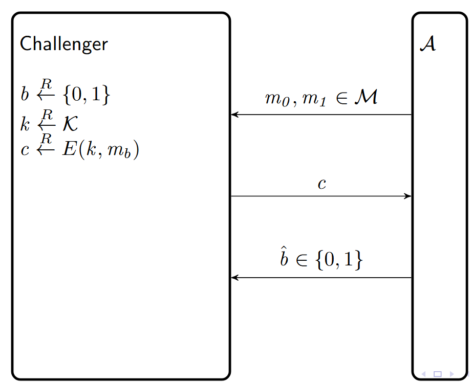
Definition:
We define $\mathcal{A}$’s bit-guessing advantage as:
Lemma:
证明:
因为b是随机挑选的,所以
那么有
根据之前$W_0,W_1$的定义可以得到:
所以:
. $\square$
Theorem 3:
The one-time pad (OTP) has indistinguishable ciphertexts.
证明:
我们用bit-guessing game来证明这个thm。
Let $\mathcal{A}$ be any adversary. Assume it outputs messages $m_0, m_1 \in \{0,1\}^L$ for some length $L$.
Since $k$ is randomly chosen, $m_b \oplus k$ is a uniformly random bitstring of length $L$, independent of $b$. 所以说只能随机猜测b。
所以
.$\square$
Secret key cryptography
Definition 10 (Pseudo-random generator):
A pseudo-random generator (PRG) is an efficiently computable function
where:
- $|\mathcal{S}| < |\mathcal{R}|$
- $\mathcal{S}$ (usually $\{0,1\}^l$) is called the
seed space. - $\mathcal{R}$ (usually $\{0,1\}^L$, $L > l$) is called the
output space.
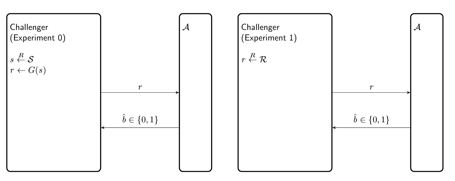
我们可以继续哟个attack game来formalize “random”的概念。
Attack Game 3 (PRG advantage):
For a given PRG $G$ defined over $(\mathcal{S}, \mathcal{R})$ and for a given adversary $\mathcal{A}$, we define two experiments.
For $b = 0,1$, Experiment $b$ proceeds as follows:
- The challenger computes $r \in \mathcal{R}$ as follows and sends it to $\mathcal{A}$:
- if $b = 0$: $s \xleftarrow{R} \mathcal{S},\ r \leftarrow G(s)$
- if $b = 1$: $r \xleftarrow{R} \mathcal{R}$
- The adversary outputs a bit $\hat{b} \in \{0,1\}$
- Let $W_b$ be the event that $\mathcal{A}$ outputs 1
图示:
Definition:
we define $\mathcal{A}$’s PRG distinguishing advantage as:
Definition 11 (Secure PRG):
A PRG $G$ is secure, if $PRGadv[\mathcal{A}, G]$ is negligible for all PPT adversaries $\mathcal{A}$.
Definition 12 (Stream Cipher Construction):
Given a PRG $G : \mathcal{K} \to \{0,1\}^L$, we define the basic stream cipher $\Pi = (E, D)$ over
$(\mathcal{K}, \{0,1\}^L, \{0,1\}^L)$ as follows:
- $E(k, m) := G(k) \oplus m$
- $D(k, c) := G(k) \oplus c$